

When a ball rolls off the end of a table it does two things at once, and the whole of projectile motion rests on the fact that these two things do not interfere with each other. Horizontally it keeps the speed it left with, because nothing pushes it forwards or backwards. Vertically it falls exactly as it would have fallen from rest, because gravity does not care that it is also moving sideways. A ball rolled gently off a bench and one fired hard off the same bench hit the floor at the same moment; only the distance out from the bench differs. This independence is what lets ballistics, long-jump technique and the trajectory of a thrown javelin be calculated at all.
The consequence is a strikingly simple prediction. The time in the air is fixed entirely by the drop height: h = ½gt² gives t = √(2h/g), the same for every launch from the same bench. The horizontal distance is then whatever that fixed time buys at the launch speed, Δx = vxt = vx√(2h/g). Range is therefore directly proportional to launch speed — not to its square, and not to anything more complicated — and a graph of one against the other is a straight line through the origin whose slope is the flight time in seconds.
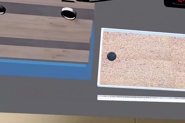
In this laboratory a metal ball is fired along a horizontal rail and off its end into a sandbox. Two photodiode sensors a fixed distance apart on the straight section of the rail time the ball as it passes, which gives the launch speed directly; the ruler gives the height of the rail above the landing surface, and a tape measure gives the range from the end of the rail to the point of impact. Eight launches are made at increasing launcher intensity, and the pairs of launch speed and range are plotted against one another. What is being tested is whether the slope of that line matches √(2h/g) computed from the measured height — a prediction made with no free parameters at all.
Educational Goals
Understanding projectile motion as two independent problems
- State and defend the claim that the horizontal and vertical motions of a projectile are independent, and use it to explain why every ball launched from the same height lands at the same instant.
- Identify which quantity fixes the time of flight and which fixes the range, and predict what happens to each when the other is changed.
Measuring a speed with a pair of sensors
- Compute the launch speed as vx = Δxsensor/Δt from the fixed sensor separation and the measured interval, and explain why this average speed is also the instantaneous speed on a straight, level section of rail.
- Judge the precision of that speed from the timer’s resolution, and recognise that the fastest launches give the shortest intervals and therefore the least precise speeds.
Applying the kinematic equations
- Derive t = √(2h/g) from h = ½gt² and combine it with Δx = vxt to obtain the range relation Δx = vx√(2h/g).
- Substitute the measured height into that expression to predict a range before the launch is made, and compare the prediction with the measurement.
Building and interpreting a graph
- Plot range against launch speed for all eight launches and test whether the points lie on a straight line through the origin.
- Interpret the slope physically — it is the time of flight in seconds — and compare it with √(2h/g) rather than treating it as an empirical fitting constant.
Evaluating errors and their direction
- Distinguish errors that can only shorten a range, such as air resistance and friction on the rail, from those that can act either way, and use that asymmetry to diagnose a systematic offset.
Relating the result to the world outside the laboratory
- Apply the same relation to a thrown ball, a jet of water or a vehicle leaving a ramp, and explain why a longer throw needs more speed in exact proportion but a higher release only as the square root.
Protocol
- Fix the 2 sensors of the stopwatch to the back of the rail on its straight section, at the location where the circular metal supports are.
- Using the ruler, measure the height of the rail as well as the distance between the sensors.
- You can adjust the intensity of the ball launcher by clicking the + and – buttons to increase and decrease the intensity.
Adjust the intensity to 1 to begin.
- Launch the metal ball along the rail by pressing the red button.
Observe the fall of the ball and measure the distance from the point of impact with the ground.
- Repeat seven more times steps 3 to 5 while adjusting the intensity of the ball launcher gradually upward.
The time interval measured by the stopwatch is recorded in the results table.
The range of the ball is recorded in the results table.
Anticipated Outcomes
Eight launches at rising intensity produce eight pairs of numbers: a sensor interval Δt, from which the launch speed follows, and a range measured from the end of the rail to the point of impact. The expected result is that range is proportional to speed. The laboratory publishes two worked examples rather than the full table — a sensor separation of 0.100 m with Δt = 0.079 s giving vx = 1.3 m/s, and a launch at vx = 2.4 m/s reaching 1.295 m — together with a drop height of h = 1.406 m. Everything below is worked from those figures; teachers should treat the predicted ranges as the model to test against their own eight measurements.
The time of flight, which is the same for every launch. Vertically the ball starts with no downward velocity, so h = ½gt² and t = √(2h/g) = √(2 × 1.406 / 9.8) = √0.2869 = 0.536 s. This is the constant the laboratory calls k, and the page’s value of 0.54 s is confirmed. Every ball in the series is in the air for 0.536 s whether it leaves the rail at 1 m/s or at 3 m/s — the single most counter-intuitive statement in the experiment, and the one most worth demonstrating by ear, since all eight impacts sound the same interval after their launches.
The range relation. Horizontally there is no acceleration, so Δx = vxt = vx√(2h/g) = 0.536 vx, with Δx in metres when vx is in metres per second. Substituting the published fast launch, Δx = 0.536 × 2.4 = 1.286 m against the 1.295 m recorded. Substituting the slow one, vx = 0.100/0.079 = 1.27 m/s and Δx = 0.536 × 1.27 = 0.68 m.
| Launch speed vx | Sensor interval Δt = 0.100 m / vx | Time of flight √(2h/g) | Predicted range 0.536 vx |
|---|---|---|---|
| 1.00 m/s | 0.1000 s | 0.536 s | 0.54 m |
| 1.27 m/s | 0.0790 s | 0.536 s | 0.68 m |
| 1.50 m/s | 0.0667 s | 0.536 s | 0.80 m |
| 2.00 m/s | 0.0500 s | 0.536 s | 1.07 m |
| 2.40 m/s | 0.0417 s | 0.536 s | 1.29 m |
| 3.00 m/s | 0.0333 s | 0.536 s | 1.61 m |
| Published trial | Sensor interval Δt | Launch speed vx = 0.100 m / Δt | Range predicted by the model | Range recorded | Difference |
|---|---|---|---|---|---|
| Slow launch | 0.079 s | 1.27 m/s | 0.68 m | not published | — |
| Fast launch | 0.042 s (implied) | 2.40 m/s | 1.286 m | 1.295 m | +9 mm (+0.7 %) |
The one published range is slightly long, and that is the wrong direction. The model gives 1.286 m for a 2.4 m/s launch and the page records 1.295 m, an excess of 9 mm. Two of the three physical effects at work here can only shorten a range: friction between the sensors and the end of the rail makes the ball leave more slowly than it was timed, and air resistance decelerates it in flight. The drag is genuinely negligible — for a 16 mm steel ball, ½ρCdAv² at 2.4 m/s is about 3 × 10⁻⁴ N against a weight of 0.16 N, giving a horizontal deceleration near 0.02 m/s² and a shortening of only about 3 mm — but it has the wrong sign for what is observed. An excess must come from somewhere else: most likely the drop height, since h enters as a square root and 9 mm of extra range corresponds to h = 1.427 m, exactly 21 mm more than the recorded value, which is about the radius of a ball plus the depth of its landing crater in sand. Measuring h from the ball’s centre at the lip of the rail to the sand’s surface, rather than from the rail to the floor, would resolve it. With one point published the discrepancy also sits inside the ±0.06 m the timer allows, so it is only worth pursuing if the same excess appears across all eight launches — in which case it is systematic and the height is the thing to re-measure.
Summary of Assignment by Grade Range
Grade 9–10
Focus: observing the pattern and recording it properly. Students set the sensors, measure the rail’s height and the sensor separation, and run all eight launches, tabulating the interval and the range each time. They convert each interval to a speed by dividing 0.100 m by it, and plot range against speed by hand. The expected conclusions are that a faster launch travels further in direct proportion — doubling the speed doubles the range — and that the graph passes through the origin, because a ball launched at no speed lands at the foot of the rail. Vocabulary: projectile, launch speed, range, time of flight, proportional.
Grade 11
Focus: the derivation and the quantitative test. Students derive t = √(2h/g) from the vertical motion, combine it with the horizontal motion to obtain Δx = vx√(2h/g), and compute the constant from the measured height: 0.536 s for h = 1.406 m. They then compare that predicted slope with the slope of their own graph, which is a real test rather than a fit, because the two come from entirely independent measurements — one from a ruler, the other from a timer and a tape. Any systematic gap between them is the result worth discussing, and its sign is informative.
Grade 12 / College Level
Focus: the projectile model across the launcher’s full range. Students derive Δx = vx√(2h/g), predict the range at each launch speed, and test the prediction against the measured ranges over the launcher’s working range. The concluding exercise is to estimate the drag on the ball explicitly (about 3 mm of shortening at 2.4 m/s for a 16 mm steel sphere) and to explain why the two published launches land where the model says they should.
Laboratory essentials
Instruments
- Electric ball launcher, with intensity settings 1 to 8
- Launch rail with two photodiode sensors (0.100 m apart)
- Metal ball
- Sandbox (landing area)
- 50 cm ruler
- Tape measure (2 m)
Products
None — this laboratory uses no chemical reagents.