
A magnet’s influence extends into the space around it, and that space can be mapped. Every compass needle that has ever pointed north has been reading such a map, drawn in this case by the Earth itself, whose molten iron core makes the planet one enormous and slightly crooked bar magnet. The same mapping underlies the read head of a hard disc, the loudspeaker in a telephone, the deflection of charged particles in a medical scanner, and the magnetic clasp on a bag. What makes the field hard to teach is that it is invisible — and what makes this laboratory work is that iron filings and a compass, between them, make it visible.
A magnetic field has a direction at every point, and the convention is to draw lines whose tangent gives that direction and whose crowding indicates the strength. Outside a magnet the lines run from the north pole to the south pole; inside the magnet they continue from south to north, so that every line closes on itself. There are no loose ends, because there is no such thing as an isolated magnetic pole: break a bar magnet in half and you get two smaller bar magnets, never a north on its own. Two lines can never cross, because the field cannot have two directions at the same place. Where two magnets are brought together their fields do not simply overlap — they add as vectors, and the result can include points where the two contributions cancel exactly.
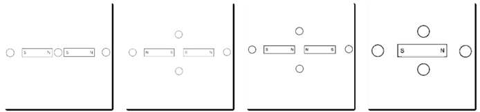
In this laboratory you will lay a magnet on a sheet strewn with iron filings and watch the filings arrange themselves along the field lines, then place a compass at marked positions around the magnet and photograph its orientation at each. You will repeat the mapping with two magnets in three further arrangements — like poles facing in setups B and C, opposite poles facing in setup D — and use the photographs to describe how two fields combine, where the field is strongest, and where between two like poles it vanishes altogether.
Educational Goals
Reading a field map
- Describe the direction of a magnetic field at a given point from the pattern the filings make, and infer the relative strength of the field from how densely they crowd.
- Explain why field lines never cross and why every line closes on itself.
Using the compass as an instrument
- Place a compass in a field and read the direction of the field from the needle, remembering that the needle’s north end points along the field.
- Explain why the filings alone cannot give the sense of the field, only its line, and why the compass is therefore not optional.
Combining two fields
- Predict the pattern produced by two magnets from the fact that fields add as vectors, before looking at the filings.
- Locate the neutral point between two like poles and say what the compass does there.
Distinguishing poles
- State which pole of the compass needle is attracted to which pole of the magnet, and reconcile that with the rule that like poles repel.
- Explain why the Earth’s geographic north attracts the north end of a compass needle, and what that implies about the polarity of the Earth’s field.
Recording and comparing
- Photograph each configuration systematically so that four compass positions in four setups can be compared afterwards rather than remembered.
- Draw the field pattern from the photographs, marking pole polarity, line direction and any neutral point.
Protocol
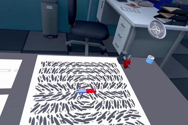
In the laboratory, it is possible to see the shape of a magnetic field by depositing iron filings around a magnet.
The small iron particles, sensitive to magnetism, naturally align along the field lines and thus trace the invisible path of the latter. But what happens if two magnets are placed close to each other?
Their fields mix and form a new pattern. One can then ask : how will the field lines organize themselves, and in which direction will the needle of a compass placed at various locations around the two magnets orient itself?
- Place a straight magnet on the iron filings sheet to reproduce setup A, with the south and north poles oriented according to the diagram.
The iron filings align according to the magnetic field produced by the magnet.
- Assembly A has 4 possible positions for the compass (illustrated by the dotted circles). Place the compass at one of the positions.
- Take a photo of the setup using the “Save Image” button on the tablet.
- Repeat steps 2 and 3 for each of the possible compass positions.
- Using 2 magnets, repeat steps 1 to 4 following setups B, C and D.
The photos of the setups will allow drawing conclusions about the magnetic fields produced by the magnets.
Anticipated Outcomes
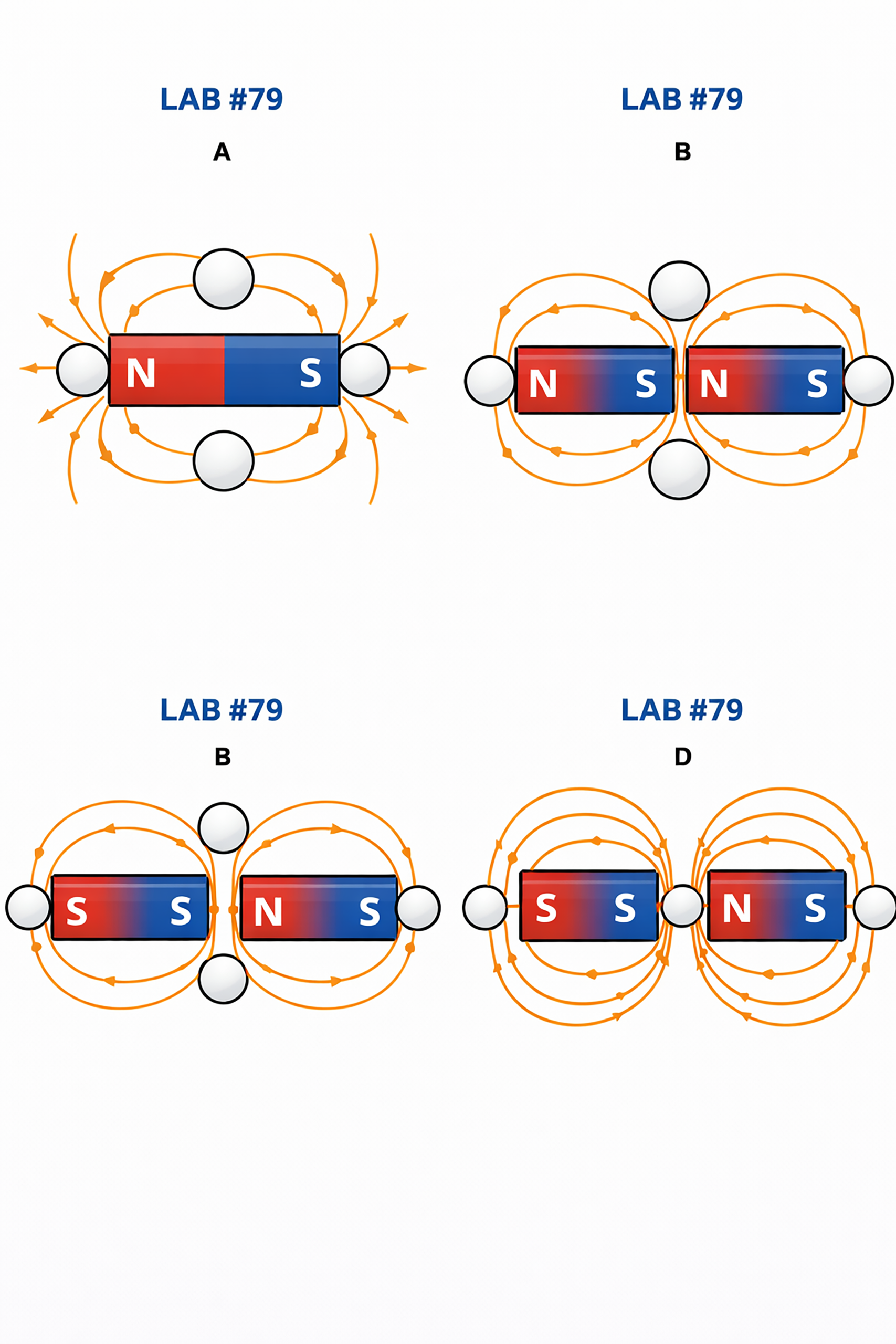
What each setup shows. The filings trace the shape of the field; the compass supplies the one thing the filings cannot, which is which way along that shape the field points. A filing is a small piece of soft iron with no polarity of its own: the field magnetises it, it becomes a tiny magnet aligned with the field, and it then chains end to end with its neighbours. Turn the magnet round and the pattern is identical, because the pattern carries no sense of direction. The compass needle is itself a permanent magnet, so it does carry one, and its north end lies along the field — which, outside the bar magnet, means it points away from the magnet’s north pole and towards its south.
| Setup | Arrangement | What the filings show | What the compass shows |
|---|---|---|---|
| A | one bar magnet | closed loops leaving the north pole and re-entering the south, densest at the two poles and sparse at the sides | at each of the four positions the needle lies tangent to the local line, its north end pointing along the field, so the four photographs together give the sense of circulation |
| B and C | two magnets with like poles facing | the lines from the two facing poles curve away from each other, leaving a clear gap between the magnets that no line crosses | approaching the midpoint the needle becomes hesitant and finally has no local field to align to — the neutral point |
| D | two magnets with opposite poles facing | the lines run straight across the gap from the north pole of one magnet into the south pole of the other, and the region between the magnets is the most densely packed on the sheet | the needle points steadily from the north pole towards the south pole all the way across the gap, and swings hardest there because the field is strongest |
Why a neutral point appears and what really happens there. Fields add as vectors. In setups B and C the two magnets are alike and face each other with like poles, so at the midpoint their contributions are equal in size and opposite in direction and they cancel exactly. That is the neutral point: the filings show it as a bare patch, because there is no field to align them, and the field lines from either side are pushed outwards around it. The usual description — that the compass there gives no clear direction — is only true of the magnets’ field. In a real laboratory the needle at a neutral point does something more interesting: with the magnets’ contribution cancelled, the only field left is the Earth’s, so the needle turns and points north, weakly and sluggishly. The neutral point is not a place where the compass fails but the one place on the sheet where it works as a compass again.
How strong are these fields. The field on the axis of a bar magnet falls off as the cube of the distance, B = (µ0/4π)(2m/r3), with µ0/4π = 10−7 T·m/A and m the magnet’s dipole moment. The cube, rather than the square familiar from Coulomb’s law, is the direct consequence of there being no isolated poles: a magnet is always a north and a south together, and at a distance their contributions very nearly cancel. Taking a laboratory bar magnet with m ≈ 0.5 A·m2 gives the figures below, against the Earth’s own field for comparison — about 54 µT in total at the latitude of Quebec, of which only some 18 µT is horizontal, the rest pointing steeply downwards.
| Distance from the pole | Field on the axis | Compared with the Earth’s horizontal field |
|---|---|---|
| 2 cm | ≈ 12 mT | 700 × |
| 5 cm | ≈ 800 µT | 45 × |
| 10 cm | ≈ 100 µT | 5.6 × |
| 15 cm | ≈ 30 µT | 1.7 × |
| 18 cm | ≈ 18 µT | 1 — the two are equal here |
| 30 cm | ≈ 4 µT | 0.2 × |
Why the needle settles where it does. A compass needle is a small dipole of moment m sitting in a field B, and the field exerts on it a torque τ = mB sin θ, where θ is the angle between the needle and the field. The torque vanishes when the needle lies along the field and is largest across it, so the needle swings, overshoots, and is brought to rest by friction at the pivot pointing along the local field line. There is a second equilibrium at 180°, which is why a needle that has been jolted can occasionally settle backwards; it is unstable, and a light tap restores it. The swinging itself is usable: the period of the small oscillations is T = 2π√(I/mB), so a needle in a strong field oscillates quickly and one at a nearly neutral point takes seconds to settle. A class with a stopwatch can turn that into a measurement of field strength without any instrument at all.
Poles, and the confusion that will not go away. Like poles repel and opposite poles attract, and the north end of the compass needle is attracted to the south pole of a bar magnet. Applied to the Earth this gives the result students find hardest to accept: since the north end of every compass needle is pulled towards the Earth’s geographic north, the magnetic pole sitting up there must be a south magnetic pole. The naming is historical — the needle’s north-seeking end was named first, and the Earth’s polarity was worked out afterwards — and it deserves saying explicitly, because otherwise the compass appears to break the rule that this laboratory is teaching. The Earth’s field is also not aligned with its rotation axis, which is why a compass in Quebec points appreciably west of true north, and it reverses every few hundred thousand years, most recently about 780 000 years ago.
Honest limits of this experiment. Nothing is measured: the record consists of photographs, so the field’s strength, the position of the neutral point and the distances of the compass positions from the magnet are all read qualitatively, and none of the figures in the table above can be checked against the laboratory as it stands. The filings show the field only in the plane of the sheet, whereas the real field fills the space above and below it, and the loops that appear to close on the paper are in fact sections through surfaces. In a physical version the sheet has to be tapped for the filings to break free of friction and settle into the pattern, a step this simulation does not require and which conceals how delicate the real demonstration is. Two further cautions for anyone reproducing this on a bench: iron filings must never be dropped directly onto a magnet, since they cannot then be removed, and the field of a magnet at a few centimetres is hundreds of times the Earth’s, so a compass that has been brought too close to a strong magnet can be permanently re-magnetised and will thereafter point the wrong way.
Summary of Assignment by Grade Range
Grade 9–10
Focus. Seeing that a field has a shape, and that a compass reads it.
Activities. Complete setup A with all four compass positions and photograph each. Sketch the pattern by hand from the photographs, marking the poles and drawing arrows on the lines from the compass readings. Then look at setups B, C and D and describe in words how each differs from A.
Expected of the student. State that field lines leave the north pole and return to the south; say where the field is strongest and give the evidence from the filings; state the rule for attraction and repulsion of poles; and explain why the compass needle turns.
Grade 11
Focus. Two fields added together.
Activities. Predict the pattern of each two-magnet setup before building it, then compare the prediction with the filings. Locate the neutral point in setups B and C and account for its position by symmetry. Compare the density of lines in the gap in setup D with the same region in setup B and explain the difference.
Expected of the student. Explain that fields add as vectors and that a neutral point is an exact cancellation, not an absence of magnets; justify why field lines never cross; describe what the compass does at the neutral point and why the Earth’s field is the answer; and relate the crowding of lines to the strength of the field.
Grade 12 / College Level
Focus. Quantitative magnetostatics and the limits of a qualitative map.
Activities. Use B = (µ0/4π)(2m/r3) to estimate the field at each compass position and to find the distance at which the magnet’s field falls to the Earth’s. Derive the torque on the needle and the period of its oscillations, and design a measurement of field strength from the oscillation period. Explain the cube law from the fact that a dipole is two opposite poles a short distance apart.
Expected of the student. Show why the field of a magnet falls off faster than that of a point charge, and connect that to the non-existence of magnetic monopoles and to ∇·B = 0; determine the position of the neutral point for two unequal magnets rather than two equal ones; and state clearly which conclusions on this page follow from the photographs and which are brought in from theory.
Laboratory essentials
Instruments
- Bar magnets (2)
- Compass (1, moved between the marked positions)
- Acrylic sheet (1)
- White paper (1 sheet)
- Tablet, for the Save Image function
- Setup diagrams A to D
Products
- Iron filings