

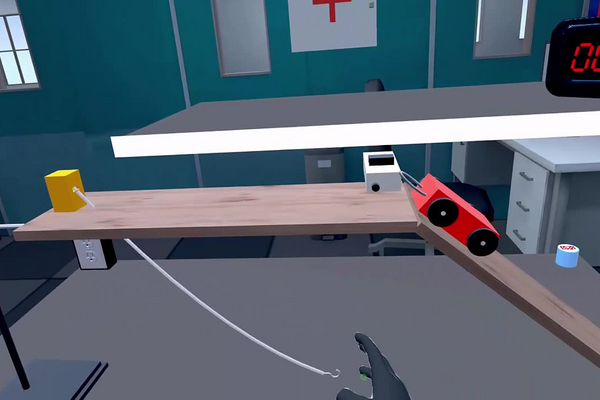
A cart released at the top of a ramp speeds up as it descends, and it does so at a rate that stays the same from the top of the board to the bottom. That is uniformly accelerated motion — the same amount of speed gained in every second — and it is the simplest case in which velocity changes. Engineers meet it wherever a load runs down a slope: gravity roller conveyors in a warehouse, a luge track, the ramp used to unload a truck. It is also the reference case against which every more complicated motion is compared.
The cause is that only part of the cart’s weight acts along the board. Gravity pulls straight down with a force mg; on a slope of angle θ the component along the surface is mg sin θ, and the component pressing the cart into the board is mg cos θ. The first drives the cart, the second sets how hard friction resists it, so the acceleration down the slope is a = g (sin θ − μ cos θ). The mass cancels out of that expression entirely: a heavy cart and a light one accelerate identically down the same ramp, although the heavy one carries more energy when it gets there.
In this laboratory you will build an inclined plane from two boards and a clamp on a universal support, run a 250 g cart down it while a spark timer prints a dot on a paper tape at fixed intervals, and repeat the descent at three increasing angles. The tape is the record of the motion: dots that grow further apart mean the cart is speeding up, and the rate at which the spacing grows is the acceleration. From that acceleration and the distance travelled you will then account for the energy — how much gravitational potential energy was released, how much of it arrived at the foot of the ramp as kinetic energy, and how much friction took on the way down.
Educational Goals
Building and characterising an inclined plane
- Assemble a stable ramp from a universal support, a clamp and two boards, and raise it in controlled steps so that only the angle changes between trials.
- Record the angle of each trial and recognise it as the single independent variable of the experiment.
Recording motion with a spark timer
- Thread the tape through the recording chronometer, attach it to the cart, and start the timer so that the descent and the record begin together.
- Read a completed tape: identify the start of the motion, measure the spacing of the dots, and explain why the spacing grows.
Measuring velocity and acceleration from data
- Calculate an average velocity over each interval as v = Δx / Δt, and treat it as the instantaneous velocity at the middle of that interval.
- Obtain the acceleration two independent ways: from the slope of a velocity–time graph, and from the constant difference between successive dot spacings.
Applying the equations of uniformly accelerated motion
- Use Δx = ½at², v = at and v² = 2aΔx to predict a descent time or a final speed before the trial is run, then compare the prediction with the tape.
- Explain why a position–time graph of this motion is a parabola while the velocity–time graph is a straight line.
Resolving forces on a slope
- Decompose the weight into the components mg sin θ along the board and mg cos θ perpendicular to it, and build the equation of motion from them.
- Extract a coefficient of friction from a measured acceleration, and predict the angle below which the cart will not start at all.
Accounting for the energy
- Compute the potential energy released (Ep = mgΔx sin θ), the kinetic energy at the foot (Ek = ½mv²) and the difference between them.
- Identify that difference as the work done against friction, Wf = ΔEm, and convert it to a force through Ff = Wf / Δx.
Judging the quality of a measurement
- Compare the size of the effect being measured with the resolution of the instrument measuring it, and group dots on the tape when a single interval is too short to resolve.
- Distinguish a random scatter that repeated trials will reduce from a systematic offset that they will not.
Protocol
- Fix a clamp to the universal support (lowest position).
- Place a first board on the end of the clamp.
- Place a second board on the end of the first so that it rests in an inclined manner.
- The value of the angle is noted in the results table.
- Position the 250g cart at the top of the inclined plane.
- Position the recording stopwatch near the junction of the two boards.
- Position the tape dispenser on the first board.
- Attach the hook to the tip of the tape dispenser to the ring of the cart.
- Start the timer. This will trigger the descent of the carriage.
- Once the cart is at the end of the board, stop the chronometer.
- The measurements of the recording chronometer are found in the results table.
- Reset the stopwatch with the right button.
- Fix the clamp to the universal support at a position just a little higher. The board will tilt with a more pronounced angle.
- Reposition the 250g cart at the top of the inclined plane.
- Activate the chronometer. This will trigger the descent of the carriage.
- Once the cart is at the end of the board, stop the chronometer.
- Reset the chronometer with the right button.
- Fix the clamp to the universal support at the highest position. The board will tilt with an even more pronounced angle.
- Repeat steps 14 to 16 with this new angle.
- From the data collected in the results table, calculate the acceleration of the cart, also perform the calculations of potential energy, kinetic energy and mechanical energy of the cart.
- Determine the magnitude of the friction force acting on the cart during its descent.
Anticipated Outcomes
The tape is the primary result. Its dots are printed at equal time intervals, so equal spacing would mean constant velocity and growing spacing means acceleration; on a uniformly accelerated descent the increase in spacing from one interval to the next is itself constant, and equal to aΔt². A student who measures the dot spacings, converts each to a velocity and plots velocity against time obtains a straight line whose slope is the acceleration. The line does not pass through the origin, because the timer is started an instant before the cart is released and the first dots are printed while the cart is still at rest.
This page carries one worked example rather than a measured data set: the three clamp positions used in the simulation, the angles they produce and the chronometer readings they give are not published, so the figures below are computed from the single example the laboratory states — an acceleration of about 0.45 m/s² on a 15° incline, with 0.63 J released and about 0.52 J lost to friction over a 1 m descent. Those three numbers are mutually consistent and they fix the coefficient of friction, which then predicts every other angle. Teachers should treat the tables as predictions to be tested against their own tape, not as readings taken from the build.
Fixing the friction from the stated example. With Δx = 1.00 m and a = 0.45 m/s², the cart arrives at v = √(2aΔx) = √(2 × 0.45 × 1.00) = 0.95 m/s carrying Ek = ½ × 0.250 × 0.95² = 0.11 J. The potential energy released is Ep = mgΔx sin θ = 0.250 × 9.8 × 1.00 × sin 15° = 0.63 J, so friction absorbed 0.63 − 0.11 = 0.52 J — exactly the figure the laboratory quotes. Dividing by the distance gives Ff = 0.52 J / 1.00 m = 0.52 N, and dividing that by the normal force mg cos θ = 0.250 × 9.8 × cos 15° = 2.37 N gives μk = 0.22. The same value follows directly from a = g (sin θ − μ cos θ): 0.45 / 9.8 = 0.0459, and (0.2588 − 0.0459) / 0.9659 = 0.220.
| Incline angle θ | sin θ | cos θ | a = g (sin θ − μ cos θ) | Time over 1.00 m | Speed at the foot |
|---|---|---|---|---|---|
| 15° | 0.259 | 0.966 | 0.45 m/s² | 2.10 s | 0.95 m/s |
| 20° | 0.342 | 0.940 | 1.33 m/s² | 1.23 s | 1.63 m/s |
| 25° | 0.423 | 0.906 | 2.19 m/s² | 0.96 s | 2.09 m/s |
| 30° | 0.500 | 0.866 | 3.03 m/s² | 0.81 s | 2.46 m/s |
The times come from Δx = ½at², rearranged as t = √(2Δx / a) — at 20°, t = √(2 × 1.00 / 1.33) = 1.23 s — and the speeds from v = at. Notice how sharply the acceleration responds: raising the ramp by five degrees, from 15° to 20°, nearly triples it. That is not because sin θ nearly triples (it grows by a third) but because the acceleration is the difference of two comparable terms. At 15° the driving term 0.259 and the friction term 0.220 × 0.966 = 0.213 very nearly cancel, leaving only 0.046 of g; a small change in the larger term is therefore a large change in the small remainder. This near-cancellation is the single most important thing to understand about the low-angle end of this experiment.
The angle below which nothing happens. The cart only starts if the driving term exceeds the friction term, that is if tan θ > μ. With μ = 0.22 that threshold is θ = arctan 0.22 = 12.4°, and the true starting threshold is a little higher still because static friction usually exceeds kinetic. The lowest clamp position must therefore produce a slope of at least about 13° or the cart will simply sit there, and the first trial of the experiment is likely to be the least reliable of the three no matter what the angle is.
| Incline angle θ | Energy released mgΔx sin θ | Kinetic energy at the foot ½mv² | Work against friction μmgΔx cos θ | Fraction delivered as motion |
|---|---|---|---|---|
| 15° | 0.63 J | 0.11 J | 0.52 J | 18 % |
| 20° | 0.84 J | 0.33 J | 0.51 J | 40 % |
| 25° | 1.04 J | 0.55 J | 0.49 J | 53 % |
| 30° | 1.23 J | 0.76 J | 0.47 J | 62 % |
The steeper ramp is the more efficient one, not the less. This table contains the result most likely to surprise, and it is the opposite of what intuition — and the previous version of this page — suggested. The energy released grows with sin θ, from 0.63 J to 1.23 J, while the work against friction is μmgΔx cos θ and therefore falls with angle, from 0.52 J to 0.47 J, because the cart presses less hard on a steeper board. A numerator that rises against a denominator term that falls gives a fraction delivered as motion that climbs steeply: 18 % at 15°, 62 % at 30°. In the general case the efficiency is 1 − μ/tan θ, which is a useful compact result: it goes to zero at the threshold angle and approaches 1 as the ramp approaches vertical.
Reading the tape, and why the dots must be grouped. A spark timer running at the usual 60 Hz prints a dot every Δt = 1/60 = 0.0167 s. On a uniformly accelerated tape the spacing grows by aΔt² from one interval to the next, which at 0.45 m/s² is 0.45 × (0.0167)² = 1.25 × 10⁻⁴ m — 0.13 mm, a quarter of what a millimetre ruler read to ±0.5 mm can resolve. Measured dot by dot the 15° tape will look like random scatter with no trend at all. The remedy is to group the dots: taking every sixth dot makes Δt = 0.100 s, and the increase per interval becomes aΔt² = 4.5 mm, comfortably measurable and about ±11 % at ruler precision. At 30° the same grouping gives 30 mm per interval of growth and a much better measurement. Grouping costs nothing, because averaging over six intervals is exactly what the interval-velocity method assumes anyway.
The whole descent is short: 2.10 s at 15° is about 126 dots at 60 Hz, and 0.81 s at 30° is only about 49. The steep trials therefore give a shorter tape with fewer points but larger, cleaner spacings, and the shallow trials the reverse. If the spark frequency of the build is not 60 Hz, every number in this paragraph scales as Δt² and must be recomputed; the frequency should be read off the instrument before the tapes are analysed.
What the friction actually is. A coefficient of 0.22 is a sliding number — wood on wood, or rubber on a dry board. A cart on wheels rolls with a coefficient of rolling resistance between about 0.01 and 0.05, five to twenty times smaller, so 0.22 cannot be the wheels alone. The rest of it is the tape: the cart drags a paper strip through the spark timer for the whole descent, and the timer’s guide and carbon disc press on that strip continuously. That retarding force does not depend on the cart’s weight or on the angle, which is why treating it as a friction coefficient is a convenient fiction rather than a physical constant — a fiction that will hold up well at one angle and drift at another. A class that runs the cart once with the tape attached and once without it, timing both, measures the tape’s share directly, and that comparison is the most valuable extension this apparatus supports.
Summary of Assignment by Grade Range
Grade 9–10
Focus: observing that the cart speeds up, and describing that in the vocabulary of motion. Students assemble the ramp, run the cart at the lowest clamp position and inspect the tape, marking where the dots begin to spread. They measure the spacing of grouped dots with the ruler, convert each group to an average speed, and plot speed against time to see a straight line. The expected conclusions are qualitative but precise: the cart gains speed steadily rather than all at once, the graph of speed against time is a line and not a curve, and raising the ramp makes the line steeper. Vocabulary to be used correctly by the end: velocity, acceleration, incline angle, friction.
Grade 11
Focus: the quantitative treatment. Students obtain the acceleration from the slope of the velocity–time graph and check it against the constant difference between successive spacings, then use Δx = ½at² to predict the descent time and compare it with the chronometer. They complete the energy account for each angle — mgΔx sin θ released, ½mv² delivered, the difference attributed to friction — and convert the friction work to a force and then to a coefficient. The target result is that the same coefficient emerges, to within measurement precision, from all three angles, and the target discussion is what it means when it does not.
Grade 12 / College Level
Focus: derivation and the friction threshold. Students derive a = g (sin θ − μ cos θ) from Newton’s second law applied along and perpendicular to the incline, show that the mass cancels, and predict the threshold angle tan θ = μ below which the cart will not start. The concluding argument is the one that separates the two contributions to the retarding force: rolling resistance scales with the normal force and the tape’s drag does not, so measuring the acceleration with and without the tape attached separates them, and the efficiency relation 1 − μ/tan θ can then be tested against angle rather than assumed.
Laboratory essentials
Instruments
- Universal support (lab stand) with clamp
- Wooden boards × 2
- Cart (250 g)
- Spark timer (recording chronometer)
- Tape dispenser with spark-timer tape
- 50 cm ruler
Products
None — this laboratory uses no chemical reagents.