110 – Kirchhoff law

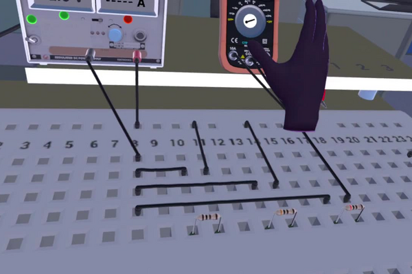
Every electrical and electronic device, from a phone charger to a national grid, is designed and diagnosed with two rules formulated by Gustav Kirchhoff in 1845. They are not new forces of nature but two conservation laws written in circuit language. Kirchhoff’s current law says that the current flowing into any junction equals the current flowing out — electric charge is conserved, so it cannot pile up at a node or vanish from one. Kirchhoff’s voltage law says that around any closed loop the voltage rises and drops sum to zero — energy is conserved, so a charge carried once around a loop returns with the energy it started with. Together with Ohm’s law they are sufficient to solve any resistor network, which is why they are the first tools of every electronics course. In this laboratory, you will put both laws to a direct experimental test. You will build a series circuit and then a parallel circuit from the same three resistors (100 Ω, 200 Ω and 300 Ω) on a 12 V supply, measure the current at every point and the voltage across every component with a multimeter, and verify that the currents at each junction and the voltages around each loop add up exactly as the two laws demand.

Educational Goals

Understanding Kirchhoff’s laws

Apply the current law (the sum of currents entering a junction equals the sum leaving) and the voltage law (the voltage drops around a closed loop sum to the supply voltage) to series and parallel circuits.
Recognise the two laws as conservation of charge and conservation of energy expressed in circuit language.

Circuit assembly

Build a series circuit and a parallel circuit from the same three resistors on a breadboard, and read component values from their colour bands.

Use of the multimeter

Measure current in series with a component and voltage in parallel across it, choosing the correct mode and connection for each.
Measure systematically: the current at every point of each circuit and the voltage across every component and the source.

Connecting theory to practice

Predict every current and voltage from Ohm’s law and the equivalent resistance before measuring, then compare prediction with measurement.

Analytical thinking

Evaluate discrepancies between calculated and measured values using percent error against the nominal value, and interpret the tolerance band as the manufacturer’s guaranteed bound on that error.

Protocol

Set up a series circuit containing the 3 resistors.
Turn on the power supply and set it to 12V.
Measure the current intensity at the output of each resistor.
Measure the intensity of the current at the source.
Measure the voltage across each resistor.
Measure the voltage at the source.
Save the circuit diagram and disassemble it.
Set up a parallel circuit containing the 3 resistors.
Repeat steps 2 to 7.

Anticipated Outcomes

Component values. Power supply 12 V. The three resistors are:

Resistor	Colour bands	Nominal value
R₁	Brown – Black – Brown – Brown	100 Ω ±1%
R₂	Red – Black – Brown – Brown	200 Ω ±1%
R₃	Orange – Black – Brown – Brown	300 Ω ±1%

First two bands give the digits, the third is the multiplier (brown = ×10) and the fourth is the tolerance (brown = ±1%).

Series circuit, steps 1 to 7. Total resistance 100 + 200 + 300 = 600 Ω, so the current is 12 V / 600 Ω = 0.020 A.

Measurement	R₁	R₂	R₃	Source
Current (step 3, step 4)	0.020 A	0.020 A	0.020 A	0.020 A
Voltage (step 5, step 6)	2 V	4 V	6 V	12 V

The current is identical at every point, and the three voltage drops sum to the supply: 2 + 4 + 6 = 12 V. This is Kirchhoff’s voltage law.

Parallel circuit, steps 8 and 9. The equivalent resistance is given by 1/R = 1/100 + 1/200 + 1/300, so R = 54.5 Ω.

Measurement	R₁	R₂	R₃	Source
Current	0.120 A	0.060 A	0.040 A	0.220 A
Voltage	12 V	12 V	12 V	12 V

Every resistor now has the full supply voltage across it, and the three branch currents sum to the source current: 0.120 + 0.060 + 0.040 = 0.220 A. This is Kirchhoff’s current law. Note that the smallest resistance carries the largest current.

Percent error. Compare each measured resistance with the value its colour bands promise, not with another measurement: percent error = (measured − nominal) / nominal × 100. The fourth band states the manufacturer’s tolerance, so a 100 Ω resistor marked ±1% is guaranteed only to lie between 99 and 101 Ω. In this simulation the components are ideal and the multimeter returns exactly the nominal value, so every percent error comes out as 0.0%. That is the correct answer here, and it is worth being explicit about why: the tolerance band is an upper bound on the error, not a prediction that an error will occur. On a physical bench the same calculation would return a small non-zero figure, and a result outside ±1% would point to a faulty component or a measurement problem rather than to normal scatter.

Series circuit analysis

Current measurements: Students will observe identical current values at all points in the series circuit, validating KCL.
Voltage measurements: The sum of voltage drops across resistors ( $V_{1} + V_{2} + V_{3}$ ) will equal the source voltage (12V), confirming KVL.

Parallel circuit analysis

Current measurements: The total current from the source will equal the sum of currents through individual resistors, upholding KCL.
Voltage measurements: Identical voltage across all parallel resistors will align with KVL predictions.

Calculations

Students will compute total resistance ( $R_{total}$ ) for both circuits and compare theoretical values (e.g., $R_{series} = R_{1} + R_{2} + R_{3}$ ) with experimental results derived from $V = I R$ .

Summary of Assignment by Grade Range

Grade 9–10

Focus: circuit behaviour as an observable pattern. Students assemble the series and parallel circuits, make the full set of current and voltage measurements, and state the two patterns in words: in series the current is the same everywhere and the voltages share the supply; in parallel the voltage is the same everywhere and the currents share the total. They distinguish the two configurations at sight and gain first proficiency with the multimeter’s two modes.

Grade 11

Focus: prediction before measurement. Students compute the equivalent resistance of each circuit (600 Ω in series; 54.5 Ω in parallel from the reciprocal sum), predict every current and voltage from Ohm’s law, and verify each junction and loop sum explicitly: 2 + 4 + 6 = 12 V and 0.120 + 0.060 + 0.040 = 0.220 A. They compute percent error against the nominal component values and read the colour bands themselves.

Grade 12 / College Level

Focus: the laws as conservation principles. Students justify the current law from conservation of charge and the voltage law from the path-independence of electric potential, derive the parallel formula from conductances, and treat the tolerance band correctly — as an upper bound on component error, not a prediction of scatter. They extend the analysis to power, verifying that the source power equals the sum dissipated in the resistors in both circuits, and note which physical resistor would need the highest power rating and why.

Laboratory essentials

Instruments

Breadboard
Resistors: 100 Ω, 200 Ω, 300 Ω (±1 %)
Connecting wires
Multimeter
Power supply (12 V)

Products

None — this laboratory uses no chemical reagents.

Watch video demo

A feel of the lab

A short capture from inside the headset showing the lab environment and protocol.

<< return to catalog